This material is provided for general informational and educational purposes only. It is not investment advice or a recommendation.
Correlation is conditional, not constant
Correlation summarizes how two return series have moved in relation to one another over a chosen period. A positive value indicates that they tended to move in the same direction, while a negative value indicates that they tended to move in opposite directions. The calculation is simple, but its interpretation is not. A historical estimate describes a particular sample of market conditions; it does not establish a permanent economic relationship.
Assets respond to multiple forces at the same time. Growth expectations, inflation, policy rates, credit conditions, currency movements and risk appetite can all influence prices. The dominant force changes from one regime to another. When the underlying shock changes, the relationship between asset returns can change with it, even if the assets themselves have not changed.
A correlation matrix is therefore better understood as a snapshot than as a structural map. It compresses a complex, time-varying system into a single set of numbers. That compression can be useful, but it can also conceal changes in the source and timing of risk.
The dominant macro shock shapes the relationship
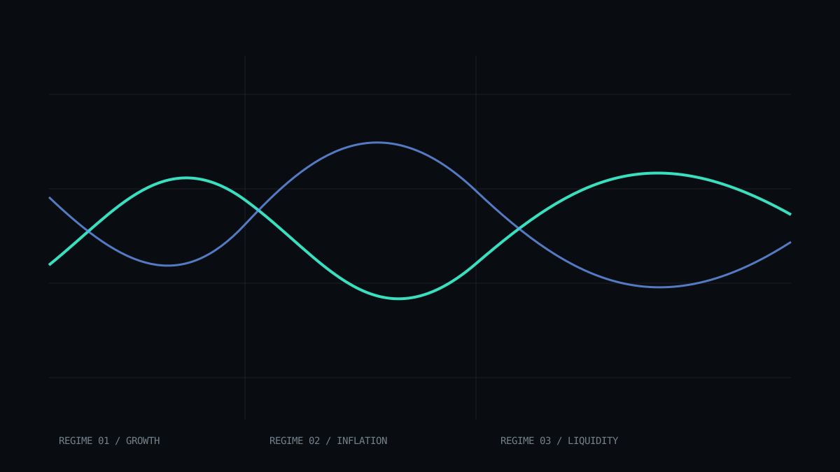
Consider the relationship between government bonds and equities. When weak growth is the central concern, disappointing economic data may lower expected corporate earnings while increasing expectations of easier monetary policy. Equity prices can fall as bond prices rise, producing negative return correlation. In that environment, duration may respond differently from growth-sensitive assets.
The relationship can reverse when inflation is the dominant shock. An upside inflation surprise may raise expected interest rates and discount rates while also pressuring corporate valuations. Bond and equity prices can then decline together, creating positive return correlation. The same pair of assets behaves differently because the market is processing a different economic disturbance.
Similar logic applies across commodities, currencies and credit. Oil can trade primarily as a signal of global demand in one period and as a supply-constrained asset in another. A currency can reflect domestic fundamentals during calm conditions but behave mainly as a funding or safe-haven instrument during stress.
Policy, positioning and market structure amplify regime shifts
Policy affects correlations through both expected cash flows and discount rates. When central banks respond aggressively to weaker activity, rates markets may offset some pressure on risk assets. When policy is constrained by inflation, that offset can weaken. Fiscal policy can also alter the mix by changing expected growth, sovereign issuance, inflation risk or the distribution of income across sectors.
Positioning can temporarily dominate economic relationships. Investors often hold similar exposures, use related risk models or face common volatility and leverage limits. A sharp move can trigger hedging, margin calls or systematic reductions in exposure across otherwise unrelated markets. During those episodes, assets may move together because balance-sheet demand becomes more important than their individual fundamentals.
Market structure matters as well. Dealer capacity, collateral availability, exchange liquidity and ownership concentration influence how shocks travel. When balance sheets are constrained, selling in one market can generate liquidity needs elsewhere. Cross-asset correlation may rise as participants sell what they can rather than only what they would prefer to sell.
Measurement choices change the reported correlation
Correlation depends on observation frequency and sample length. Daily returns may reveal short-lived risk-off episodes that are muted in monthly data. A multi-year window may blend several regimes into an apparently stable average, while a short window may be dominated by one event. Neither estimate is automatically superior; each answers a different question.
Nonlinear relationships create another limitation. Two assets may appear weakly correlated in normal markets yet move closely together during large losses. A single Pearson correlation can miss asymmetry, tail dependence or delayed transmission. Currency effects, market-closing times and stale prices can further distort cross-market comparisons.
Changes in volatility also affect interpretation. A modest correlation during a high-volatility period can represent larger joint price movements than a stronger correlation during a quiet period. Correlation therefore does not measure total risk by itself. Covariance, volatility, drawdown behavior and exposure size provide additional context.
A disciplined reading of correlation
Correlation analysis is most informative when paired with an explanation of the regime behind the numbers. Relevant questions include which macro variable is driving prices, whether policy is reinforcing or offsetting the shock, how leveraged market participants are and whether liquidity is broadly available. These questions connect a statistical relationship to an economic mechanism.
It is useful to distinguish strategic relationships from tactical co-movement. Structural links can persist over long horizons, but cyclical forces may overwhelm them for months or years. Stress episodes can create still shorter bursts of unusually high correlation. Treating all three horizons as equivalent can produce a false sense of precision.
The central lesson is not that historical correlation lacks value. It is that correlation is a state-dependent output of a changing system. Understanding why it changed is usually more informative than observing that it changed.